Mapping & Navigation

Summary

Estimated time to completion: 2 hours

Simulated robot: Turtlebot 3 Burger

What will you learn with this unit?

Simulating a robot with Gazebo and ROS
Kinematic Models: Moving a robot by publishing on topics
Creating a map of the simulated environment using 2D-SLAM
Using the Advanced Monte Carlo Localization AMCL and the ROS map server
Overview of autonomous navigation with 2D maps using the move base stack

Robot Simulation with Gazebo

We start by launching the simulations provided by Robotis.

bash

roslaunch turtlebot3_gazebo turtlebot3_world.launch

Next, we need to bring up the coordinate frame transformations.

bash

roslaunch turtlebot3_bringup turtlebot3_remote.launch

You should see the following window pop up:

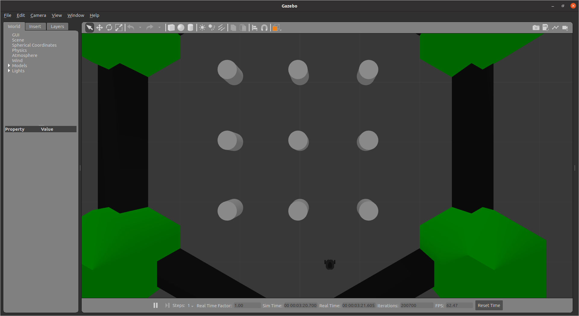
Exercise [5 min]

Inspect the running nodes and topics
Visualize the robot model and the laser scan data in Rviz

Moving a Robot by Publishing on a Topic

Mobile Robot Locomotion

We will now briefly discuss mobile robot locomotion and forward kinematics.

The term "robot locomotion" refers to the various strategies that robots use to move from one location to another. In this unit, we focus on wheeled mobile robots. Unlike industrial robots, mobile robots change their pose based on wheel motion. The pose $\vec{\xi}_t$ of our robot in the world is thus a function over time and not a function of current angular joint values. The mathematics of forward kinematics (and inverse kinematics, as we will see in the next chapter) is similar to industrial robot kinematics.

The locomotion of mobile robots is based on kinematic assumptions summarized in a "model". In this unit, we analyze and derive kinematic models for mobile robots. Initially, we start considering the most simple mobile robot: a driven wheel.

Consider a simple wheel on a plane. This wheel has a radius r. If the wheel rotates $\Delta \Phi$ , the distance moved by the center of the wheel is $\rho$ . This can be described by the equation:

$\rho = \Delta \varphi \cdot r$

Where $\rho$ is the motion of the wheel center.

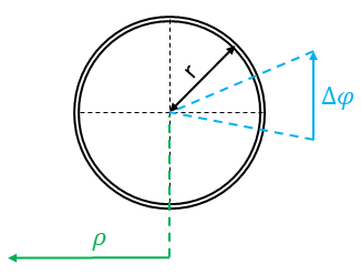
Simple wheel on a plane

However, this mobile robot would be somehow useless because it cannot change the orientation. It can only move along the direction of $\rho$ . Thus, the next step is the extension of this simple wheel model: we add a second wheel and connect the wheels. This model is called a differential-driven mobile robot, and it is the most important model for mobile robotics. A 3D sketch of the model and a 2D simplification is visible in the figure below:

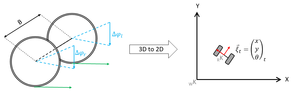
3D model (left) | Simplified 2D model (right)

In the figure on the left side, you see the 3D model. Two wheels are connected with a so-called baseline with length B. Notice that robots, like the one above, are differential mobile robots. This is only true if they have two differently controlled wheels that are in alignment. Based on the wheel movement $\Delta \varphi_l$ and $\delta \varphi_r$ , the mobile device is now able to move on a plane. Since the third dimension is not used, a mobile robot is typically controlled on a 2D plane (the top view, see the right part of the figure above).

In the two-dimensional space, the mobile robot is controlled in a world coordinate system/frame $wK$ .

The pose $\vec{\xi}_t = (x, y, \theta)^T_t$

at time t is defined in the world frame. However, the wheel motion is described in the wheel coordinate system and can be projected into the robot coordinate system _RK (see red coordinate system) using the kinematic configuration.

Now, it should be obvious that the pose $\vec{\xi}_t$ at t must be somehow a function of the wheel motion and the previous pose $\vec{\xi}_{t-1}$ . In this section, we will derive functions mapping motion from the world coordinate system to the wheel coordinate system and vice versa.

Deriving the Change of Pose

In this unit, we will only work with differential drive or holonomic mobile robots. Let us continue with the derivation of the change of pose $\vec{\xi}_t$ to $\vec{\xi}_{t+1}$ . Consider the following image.

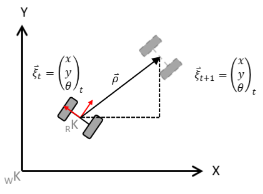
Simplified Kinematic Model of the Mobile Robot

Thus we define the robot state and want to calculate the new state $\vec{\xi}_t = (x, y, \theta)$ based on the motion of the left wheel $\Delta \varphi_l$ and the right wheel $\Delta \varphi_r$ .

As we can see, the robot will move $||\vec{\rho}||$ meters. The X- and Y-components of $~\vec{\rho}$ have to be estimated based on the latest orientation of the robot (e.g. $\delta_t$ ) and the change of orientation. This change of the robot's orientation, as well as $~||\vec{\rho}||$ , are functions of the wheel motion.

The driven distance:

$||\vec{\rho}|| = \frac{\delta_t (\Delta \varphi_l + \Delta \varphi_r)}{2}$

The change in orientation:

$\delta \theta = \frac{\delta_t (\Delta \varphi_l - \Delta \varphi_r)}{B}$

(Where B is the baseline — the distance between the wheels). Based on these calculations, the movement of the robot can be determined. For this calculation, we must know the previous pose $\vec{\xi}_{t-1}$ . Accumulating the robot's motion leads to the new pose. To calculate this, we "split" the motion $||\vec{\rho}||$ into the X and Y components.

This is simply done by using sine and cosine:

$\vec{\xi}_{t+1} = \vec{\xi}_t + \begin{pmatrix} \Delta X \\ \Delta Y \\ \Delta \theta \end{pmatrix} = \vec{\xi}_t + \begin{pmatrix} ||\vec{\rho}|| \cos(\theta_t + \Delta \theta) \\ ||\vec{\rho}|| \sin(\theta_t + \Delta \theta) \\ \Delta \theta \end{pmatrix}$

However, the equation has a shortcoming: it assumes a linear movement of the robot, but it is sufficient for our purposes. A more exact solution will be discussed in a different unit.

Forward Kinematics in ROS

Now that we know how to calculate the forward kinematics of a differential drive mobile robot, let's see how we implement it using ROS. (Remember that we already moved the TurtleBot in the previous unit in the move_turtlebot.py file).

In the following example, we will create a node that moves the robot to a specific pose referenced to the starting pose of the robot:

Simple Goal Mover in ROS

In this example, we'll implement a simple goal mover using ROS. The robot will move to a specified position in a simulated Gazebo environment.

python

#!/usr/bin/python3
import rospy
from nav_msgs.msg import Odometry
from tf.transformations import euler_from_quaternion
from geometry_msgs.msg import Point, Twist
from math import atan2, sqrt, hypot

class SimplePose:
    def __init__(self):
        """Initializes the class member variables"""
        self.x = 0.0
        self.y = 0.0
        self.theta = 0.0
        self.goal_tolerance = 0.2
        self.sub = rospy.Subscriber("/odom", Odometry, self.odom_callback)
        self.pub = rospy.Publisher("/cmd_vel", Twist, queue_size=1)
        # Waits for a message on the /odom topic to ensure the simulation has started
        rospy.wait_for_message("/odom", Odometry, 10)

    def odom_callback(self, msg):
        """Callback function to update the robot's position based on odometry data"""
        self.x = msg.pose.pose.position.x
        self.y = msg.pose.pose.position.y
        rot_q = msg.pose.pose.orientation
        (_, _, self.theta) = euler_from_quaternion([rot_q.x, rot_q.y, rot_q.z, rot_q.w])

    def go_to(self, goal_point):
        """Moves the robot towards the goal point"""
        speed = Twist()
        rho = float('inf')  # Initially set to a very large number

        while rho > self.goal_tolerance:
            delta_x = goal_point.x - self.x
            delta_y = goal_point.y - self.y
            rho = sqrt(delta_x ** 2 + delta_y ** 2)
            rospy.loginfo_throttle_identical(1, f"Distance to goal= {rho:.2f}m")
            angle_to_goal = atan2(delta_y, delta_x)

            if abs(angle_to_goal - self.theta) > 0.1:
                speed.linear.x = 0.0
                speed.angular.z = 0.3
            else:
                speed.linear.x = 0.22
                speed.angular.z = 0.0
            self.pub.publish(speed)
            rospy.sleep(0.01)

    def stop_robot(self):
        """Stops the robot's movement"""
        speed = Twist()
        speed.linear.x = 0.0
        speed.angular.z = 0.0
        self.pub.publish(speed)

if __name__ == '__main__':
    rospy.init_node("speed_controller")
    simple_pose_mover = SimplePose()

    goal = Point()
    goal.x = 5
    goal.y = 5

    try:
        simple_pose_mover.go_to(goal)
    except (KeyboardInterrupt, rospy.ROSException) as e:
        rospy.logerr(e)
    finally:
        simple_pose_mover.stop_robot()
        position_error = hypot(goal.x - simple_pose_mover.x, goal.y - simple_pose_mover.y)
        rospy.loginfo(f"Final position error: {position_error:.2f}m")

Explanation

Class Initialization: We define the SimplePose class, which initializes subscribers and publishers for the /odom and /cmd_vel topics.
Odometry Callback: This method updates the robot's current position (x, y, and theta) using the odometry data.
Move to Goal: In the go_to method, we calculate the distance (rho) and angle to the goal. If the robot is not facing the correct direction, it will rotate until aligned, then move straight.
Stopping the Robot: After reaching the goal, the robot stops.

Exercise [10 min]

Create a launch file with the name simulation2.launch that:

spawns the turtlebot3 burger in an empty gazebo world at position x=0, y=0
starts all TFs for the turtlebot3 burger
starts the just now created simple_pose.py and try to understand the code
comment the functions in the simple_pose.py so that you understand what is happening

Exercise Solution

We can launch the TurtleBot in Gazebo and test this script using the following launch file simulation2.launch.

xml

<launch>
    <include file="$(find turtlebot3_gazebo)/launch/turtlebot3_empty_world.launch">
        <arg name="model" value="burger"/>
        <arg name="x_pos" value="0.0"/>
        <arg name="y_pos" value="0.0"/>
    </include>

    <include file="$(find turtlebot3_bringup)/launch/turtlebot3_remote.launch"/>

    <node name="simple_pose" pkg="first_pkg" type="simple_pose.py" output="screen"/>
</launch>

Discussion As you probably have noticed the developed code is not realy working well. Let's change this by implementing a direct controller based on the angle and distance to the goal. For this update the init function and the go_to functions as depicted below:

python

def __init__(self):
    """Initializes the class member variables
    """
    self.x = 0.0
    self.y = 0.0
    self.theta = 0.0
    self.goal_tolerance = 0.02

    self.max_vel=0.22
    self.max_omega = 2.84

    self.k_rho = 0.3
    self.k_alpha = 0.8


    self.sub = rospy.Subscriber("/odom", Odometry, self.odom_callback)
    self.pub = rospy.Publisher("/cmd_vel", Twist, queue_size=1)
    # we wait for a message on the odom topic to make sure the simulation is started
    rospy.wait_for_message("/odom", Odometry, 10)


def go_to(self, goal_point):
    """Calculates the current distance (rho) to the goal_point as well as the angle to the goal.
    Based on the delta angle to the goal this function decides wether to rotate the robot in place or go straight ahead.

    Args:
        goal_point (Point): [description]
    """
    speed: Twist = Twist()
    rho = 999999999999999999

    while rho > self.goal_tolerance:
        delta_x = goal_point.x - self.x
        delta_y = goal_point.y - self.y
        rho = sqrt(delta_x**2 + delta_y**2)
        rospy.loginfo_throttle_identical(1, "Distance to goal= {}m".format(rho))
        angle_to_goal = atan2(delta_y, delta_x)

        alpha = angle_to_goal - self.theta

        v = self.k_rho * rho
        omega = self.k_alpha * alpha

        speed.linear.x = v if v <= self.max_vel else self.max_vel
        speed.angular.z = omega if omega <= self.max_omega else self.max_omega
        self.pub.publish(speed)
        rospy.sleep(0.01)

Mapping

Mapping describes the process of generating a useable map. In ROS this map is described using two files:

An image: The discretized map is described using pixels. A white pixel is free, a gray is unknown and a black is occupied
A yaml description file: This file describes the maps hyperparameters such as square meters per pixel

In this unit, we use the gmapping algorithm. This piece of software subscribes to two topics:

Obviously, the gmapping ROS node needs the topic of the laserscaner. Typically, your robot will publish a "\scan_description>\scan" (e.g.: "\front_scan\scan") topic. Since gmapping waits for the "\scan" topic, you have to remap. As you already know, the TF in ROS is used to coordinate the coordinate systems. To be able to transform the laserscan data to the robot's current pose, the TF tree must contain a complete description of the robot's joints as well as the sensor coordinate systems. Additionally, a TF from a world coordinate system to the current robot pose (typically named "\odom") must exist.

After the topics of gmapping were remapped, the node publishes a map. The default hyperparameters of the algorithm are typically good enough for our purpose. Initially, the map will look like the following sketch:

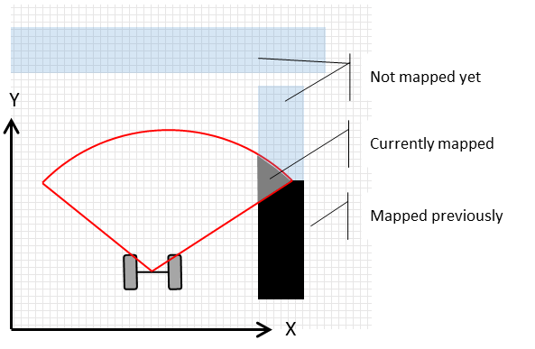
The map will be created during manual robot movement (of course, there are solutions for autonomous map creation). Depending on your system, a ROS keyboard control is enought for this task.The map will be created during manual robot movement (though autonomous solutions for map creation also exist). Depending on your system, ROS keyboard control may be enough for this task.

Additional Information

As mentioned previously, modern mobile robotics heavily relies on statistics. The gmapping ROS package is a SLAM (Simultaneous Localization and Mapping) application. In SLAM, we estimate both the current robot pose $\vec{x}_t$ and the map $m$ . This estimation is based on the knowledge gathered so far — movement commands $\{ \vec{u}_1, \dots, \vec{u}_t \}$ and measurements $\{ \vec{z}_1, \dots, \vec{z}_t \}$ . This is summarized by the probability distribution:

$p(\vec{x}_t, m \mid \vec{u}_{1:t}, \vec{z}_{1:t})$

Gmapping Demo

We will use the existing TurtleBot3 simulation in Gazebo provided by ROBOTIS. Execute the following commands in separate terminals:

Start the simulation in Gazebo and spawns the robot in the world

bash

roslaunch turtlebot3_gazebo turtlebot3_world.launch

Starts the gmapping-based SLAM for the TurtleBot3 We use a preconfiguerd launch file wich inclues a preconfigured rviz file. However you can also click together your own vizualization in rviz.

bash

roslaunch turtlebot3_slam turtlebot3_slam.launch slam_methods:=gmapping

Now drive the robot around to create the map. To enable teleoperation, you can run the following command:

bash

 roslaunch turtlebot3_teleop turtlebot3_teleop_key.launch

Alternatively, you could use rqt_robot_steering for control.

bash

rosrun rqt_robot_steering rqt_robot_steering

Let's save our map in a folder named maps inside our package first_pkg with the name my_map. Make a foder called maps in the first_pkg package:

bash

mkdir -p $(rospack find first_pkg)/maps

Move to the home directory:

bash

cd

Give the user permission to the folders:

bash

sudo chown -R  fhtw_user catkin_ws

bash

rosrun map_server map_saver -f "$(rospack find first_pkg)/maps/my_map"

Exercise [5 min]

Move the robot using any teleoperation method we've discussed so far.
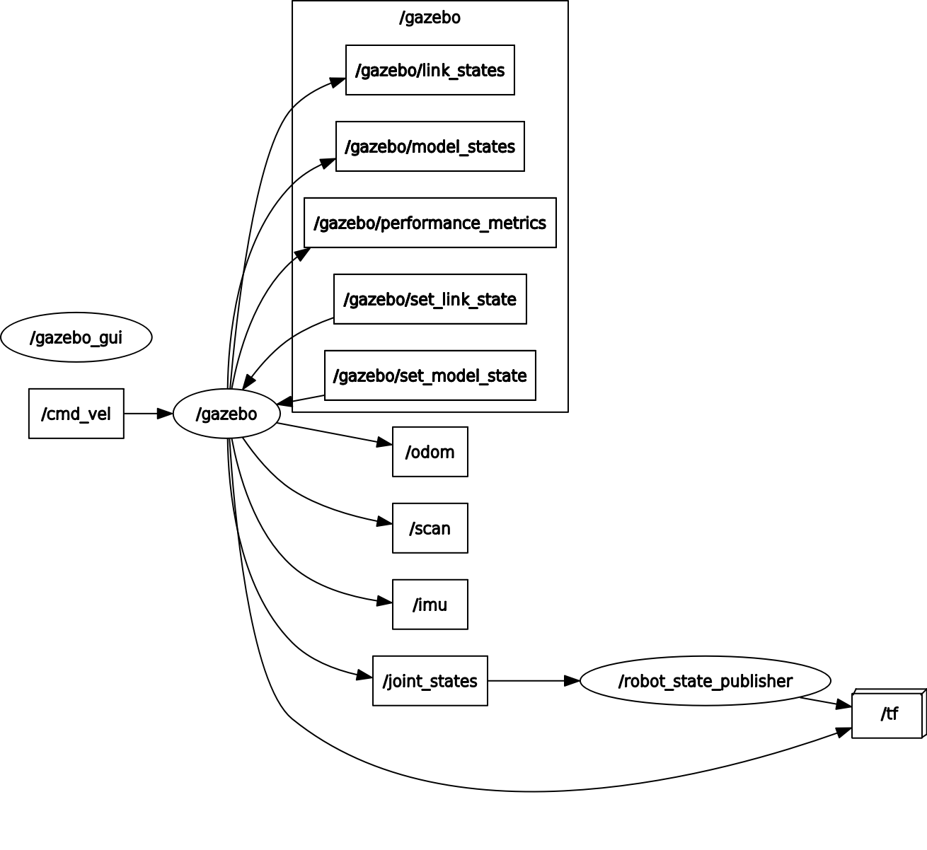
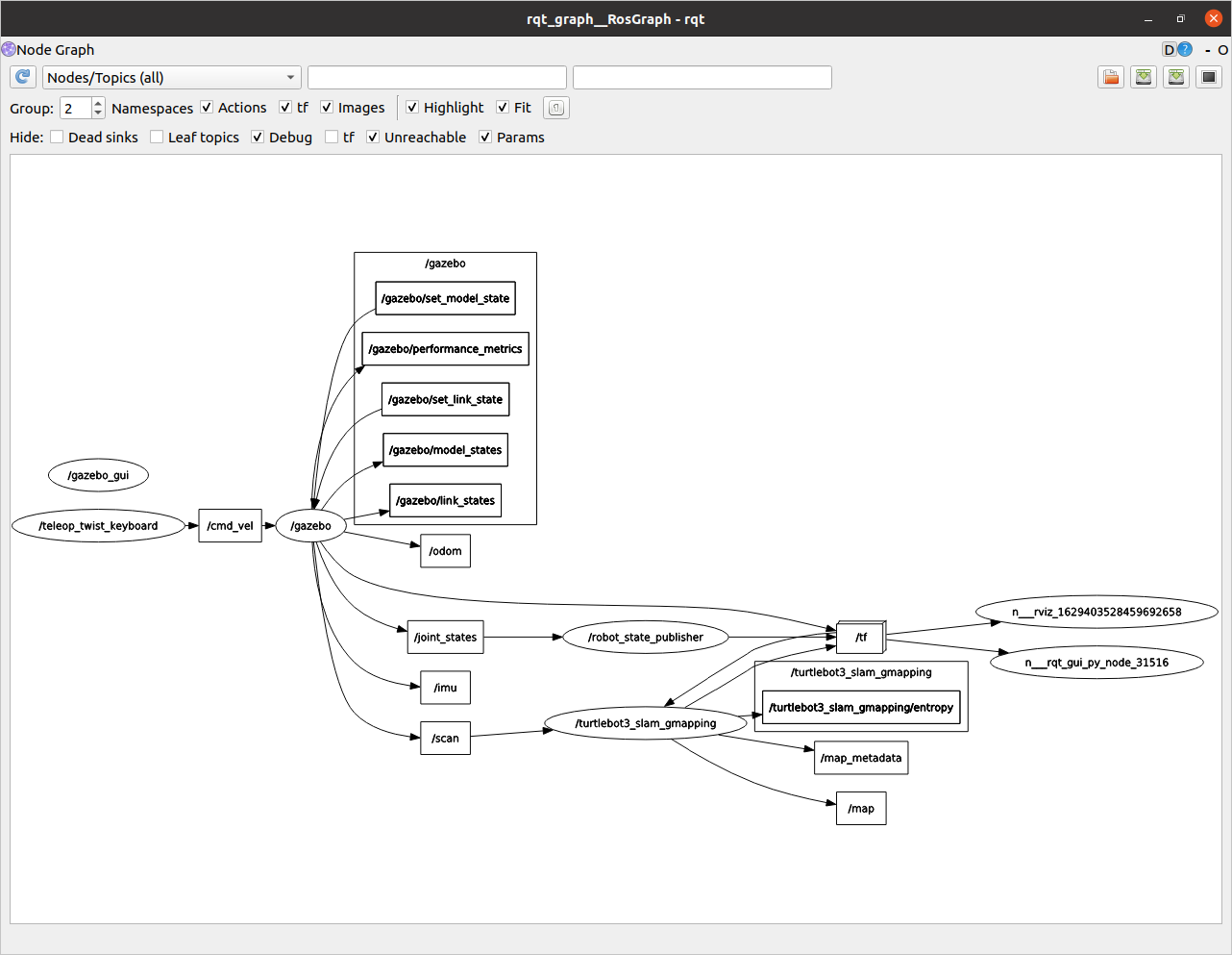
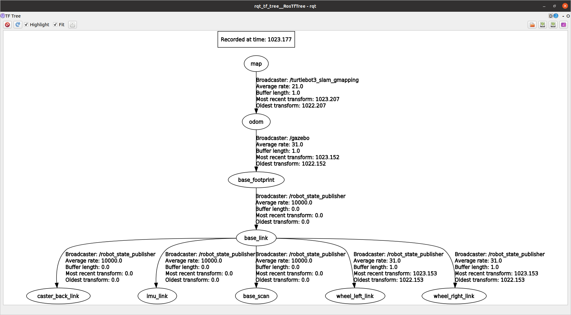
Inspect the TF tree and rqt_graph. What do you observe?
Create a complete map of the environment.
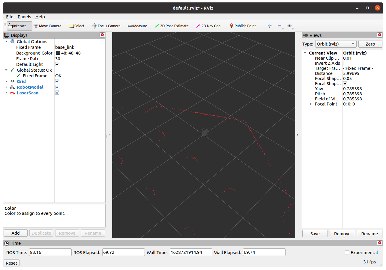
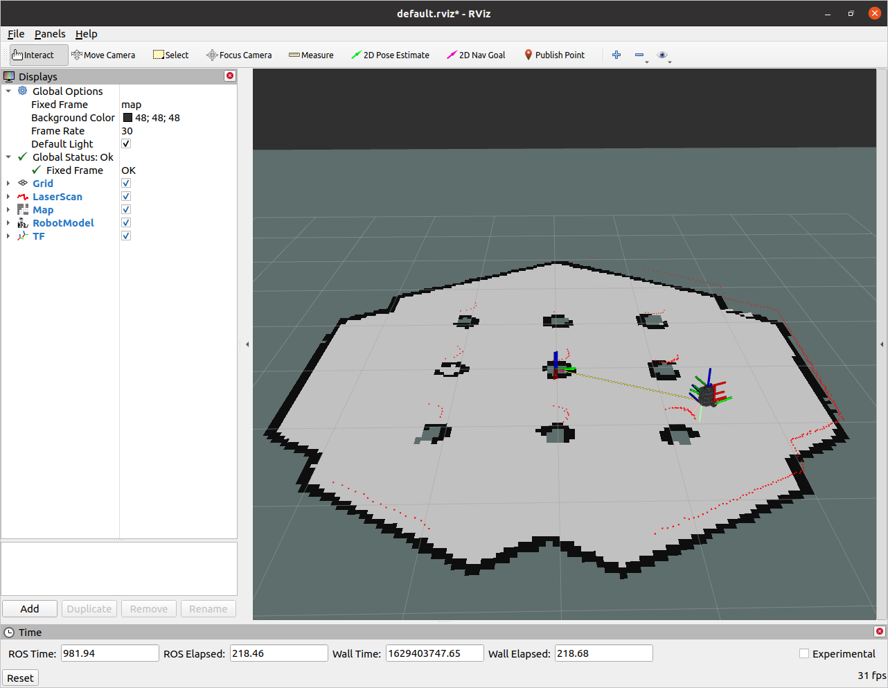
Open RVIz and visualize the following:
- Robot model
- TFs (without names)
- Laser scan data
- The map created by gmapping

Refer to the following figures for the desired output in RVIz.

Now that we know how to create a map, let's look into how to save it for later.

Map Server

The map_server provides utilities to create the YAML and image file.

The syntax is:

bash

rosrun map_server map_saver [--occ <threshold_occupied>] [--free <threshold_free>] [-f <mapname>] map:=/your/costmap/topic

Exercise [1 min]

Inspect the generated YAML file.

Exercise Solution

bash

cat $(rospack find first_pkg)/maps/my_map.yaml

image: /home/username/catkin_ws/src/JupyterROS/Basic_ROSpy/first_pkg/maps/unit3_map.pgm
resolution: 0.050000
origin: [-10.000000, -10.000000, 0.000000]
negate: 0
occupied_thresh: 0.65
free_thresh: 0.196

Localization

Localization Using AMCL

You have already learned the principles of mobile robot localization using wheel motion and kinematics. We have also discussed the issue of noisy data, but we have not found a full solution for the process and sensor noise. Without delving into deeper topics (which are part of the master degree program "Master in Robot Engineering"), we can formulate the main problem: it is not possible to describe robot motion and the robot's state using classic statistical models, such as multivariate Gaussian distributions.

Instead of using parametric probability density functions to describe the robot's state and motion, we can use a technique from statistical physics called Markov Chain Monte Carlo (MCMC). MCMC uses many (typically more than 500) samples or potential hypotheses of the robot's state, referred to as "particles". This approach is known as a particle filter. The method can be simplified into two main steps:

Sampling: Each particle is moved according to a noisy motion command. For example, using noisy motion data, we estimate each particle's movement using kinematics. Each particle moves in accordance with the real physical movement. Next, we evaluate each particle using sensor signals (e.g., checking if the motion is consistent with sensor values, like those from an accelerometer) in a probabilistic framework. This results in a set of moved particles, each weighted by the sensor data.
Resampling: Imagine you have a bag of colored balls — two red and eight blue. The probability of drawing a red ball is 20%. If you sample "with replacement" (putting the ball back after each draw), you should draw a red ball 20% of the time. In resampling, particles are selected based on their weight (better particles are sampled more often). This creates a "survival of the fittest" scenario, where the best hypothesis of the robot's state survives.

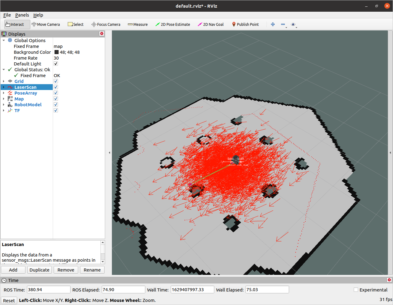
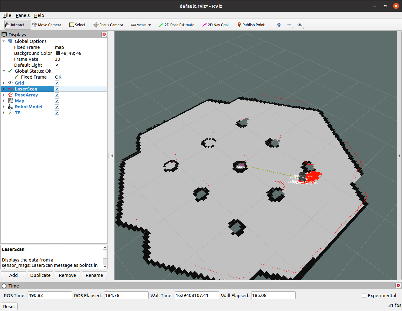
The following figure illustrates a particle filter application for robot localization. Each arrow represents a particle, with the starting point representing the robot's position and the arrow's direction indicating orientation (length is not significant).

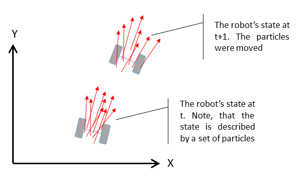
Sketch of Particle Filter in ROS

The particle filter is the default localization algorithm. As shown in the figure above, particles spread further from the "ground truth" over time. To correct this, global information (e.g., maps) is used.

References:

C.M. Bishop; Pattern Recognition and Machine Learning; Springer, 2006
S. Thrun, W. Burgard & D. Fox; Probabilistic Robotics (Intelligent Robotics and Autonomous Agents series); The MIT Press, 2005

AMCL Demo

We will now use the AMCL particle filter with the map we created. Start everything except for the mapping:

Starts simulation in Gazebo with the robot inside

bash

roslaunch turtlebot3_gazebo turtlebot3_world.launch

Starts the navigation stack with the created map passed in.

bash

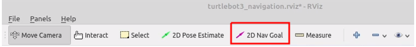
roslaunch turtlebot3_navigation turtlebot3_navigation.launch map_file:=$(rospack find first_pkg)/maps/my_map.yaml

At the beginning the robot doesn't know where it is. You can help the robot by setting an initial pose estimate in RViz. This is done by clicking the "2D Pose Estimate" button and dragging the arrow where the robot actually is.

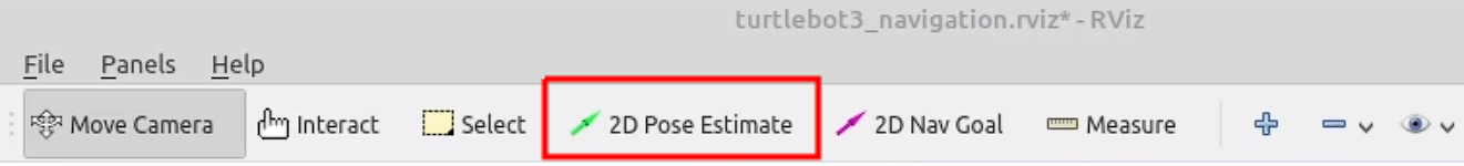
Now the robot will localize itself. Now let the robot do the work for you. You can use the 2D Nav Goal button in RViz to set a goal for the robot. The robot will move to the goal and localize itself better with each resampling step.

AMCL Launchfile

The AMCL Demo was very TurtleBot specific. However you can configure everything by yourself:

Make a rviz folder in the first_pkg package:

bash

mkdir -p $(rospack find first_pkg)/rviz

Create a new file called rviz_config.rviz in the rviz folder:

bash

touch $(rospack find first_pkg)/rviz/rviz_config.rviz

In RViz, display the following:

Robot Model
Laser Scan
TFs (without names)
map
PoseArray

Make a new launchfile called amcl.launch in the first_pkg package:

bash

touch $(rospack find first_pkg)/launch/amcl.launch

Paste the following code into the launch file:

xml

<launch>
    <!-- Start Gazebo with Turtlebot3 -->
    <!--launch world-->
    <include file="$(find gazebo_ros)/launch/empty_world.launch">
        <arg name="world_name" value="$(find turtlebot3_gazebo)/worlds/turtlebot3_world.world"/>
        <arg name="paused" value="false" />
        <arg name="use_sim_time" value="true" />
        <arg name="gui" value="false" />
        </include>

    <!--find robot description-->
    <param name="robot_description" command="$(find xacro)/xacro --inorder $(find turtlebot3_description)/urdf/turtlebot3_burger.urdf.xacro" />

    <!--spawn robot-->
    <node name="spawn_urdf" pkg="gazebo_ros" type="spawn_model" args="-urdf -model turtlebot3_burger -x -2 -y 0 -z 0 -param robot_description" />

    <!--launch remote-->
    <include file="$(find turtlebot3_bringup)/launch/turtlebot3_remote.launch"/>
    
    <!--start map server-->
    <node name="map_server" pkg="map_server" type="map_server" args="$(find first_pkg)/maps/my_map.yaml"/>
    
    <!-- Include Turtlebot movebase -->
    <include file = "$(find turtlebot3_navigation)/launch/move_base.launch" />

    <!-- Start RViz with a specific config -->
    <node pkg="rviz" type="rviz" name="rviz" args="-d $(find first_pkg)/rviz/rviz_config.rviz" />

</launch>

Now launch the file:

bash

roslaunch first_pkg amcl.launch

If you choose Fixed Frame: base_footprint in RViz, you will see the robot's pose. You may have noticed that the map is somewehere else. That's becasue the robot doesn't know where it is and there is No transform from [map] to [base_footprint]. You could calculate that with a fixed Transformation, but there is a better way. We will now use the AMCL algorithm to localize the robot. So add the AMCL node to the amcl.launch file:

xml

<launch>
    <!-- Start Gazebo with Turtlebot3 -->
    <!--launch world-->
    <include file="$(find gazebo_ros)/launch/empty_world.launch">
        <arg name="world_name" value="$(find turtlebot3_gazebo)/worlds/turtlebot3_world.world"/>
        <arg name="paused" value="false" />
        <arg name="use_sim_time" value="true" />
        <arg name="gui" value="false" />
        </include>

    <!--find robot description-->
    <param name="robot_description" command="$(find xacro)/xacro --inorder $(find turtlebot3_description)/urdf/turtlebot3_burger.urdf.xacro" />

    <!--spawn robot-->
    <node name="spawn_urdf" pkg="gazebo_ros" type="spawn_model" args="-urdf -model turtlebot3_burger -x -2 -y 0 -z 0 -param robot_description" />

    <!--launch remote-->
    <include file="$(find turtlebot3_bringup)/launch/turtlebot3_remote.launch"/>
    
    <!--start map server-->
    <node name="map_server" pkg="map_server" type="map_server" args="$(find first_pkg)/maps/my_map.yaml"/>
    
    <!-- Include Turtlebot movebase -->
    <include file = "$(find turtlebot3_navigation)/launch/move_base.launch" />

    <!-- Start RViz with a specific config -->
    <node pkg="rviz" type="rviz" name="rviz" args="-d $(find first_pkg)/rviz/rviz_config.rviz" />

     <!-- AMCL Configuration -->
    <node pkg="amcl" type="amcl" name="my_amcl_node">
        
      <param name="min_particles"             value="200"/>
      <param name="max_particles"             value="1000"/>
      <param name="kld_err"                   value="0.02"/>
      <param name="update_min_d"              value="0.20"/>
      <param name="update_min_a"              value="0.20"/>
      <param name="resample_interval"         value="1"/>
      <param name="transform_tolerance"       value="0.5"/>
      <param name="recovery_alpha_slow"       value="0.00"/>
      <param name="recovery_alpha_fast"       value="0.00"/>
      <param name="initial_pose_x"            value="-1.5"/>
      <param name="initial_pose_y"            value="0.5"/>
      <param name="initial_pose_a"            value="0"/>
      <param name="gui_publish_rate"          value="50.0"/>
        
      <remap from="scan"                      to="scan"/>
      <param name="laser_max_range"           value="3.5"/>
      <param name="laser_max_beams"           value="180"/>
      <param name="laser_z_hit"               value="0.5"/>
      <param name="laser_z_short"             value="0.05"/>
      <param name="laser_z_max"               value="0.05"/>
      <param name="laser_z_rand"              value="0.5"/>
      <param name="laser_sigma_hit"           value="0.2"/>
      <param name="laser_lambda_short"        value="0.1"/>
      <param name="laser_likelihood_max_dist" value="2.0"/>
      <param name="laser_model_type"          value="likelihood_field"/>
        
      <param name="odom_model_type"           value="diff"/>
      <param name="odom_alphal"               value="0.1"/>
      <param name="odom_alpha2"               value="0.1"/>
      <param name="odom_alpha3"               value="0.1"/>
      <param name="odom_alpha4"               value="0.1"/>
      <param name="odom_frame_id"             value="odom"/>
      <param name="base_frame_id"             value="base_footprint"/>
    </node>
</launch>

Now let the robot drive to a goal. The robot will move to the goal and localize itself better with each resampling step.

Exercise Solution

Visualization of Advanced Monte Carlo Localization

If you you can't manage to set up rviz correctly, you can copy the content premade rviz_config file below:

yaml

Panels:
  - Class: rviz/Displays
    Help Height: 78
    Name: Displays
    Property Tree Widget:
      Expanded:
        - /Global Options1
      Splitter Ratio: 0.5
    Tree Height: 354
  - Class: rviz/Selection
    Name: Selection
  - Class: rviz/Tool Properties
    Expanded:
      - /2D Pose Estimate1
      - /2D Nav Goal1
      - /Publish Point1
    Name: Tool Properties
    Splitter Ratio: 0.5886790156364441
  - Class: rviz/Views
    Expanded:
      - /Current View1
    Name: Views
    Splitter Ratio: 0.5
  - Class: rviz/Time
    Name: Time
    SyncMode: 0
    SyncSource: LaserScan
Preferences:
  PromptSaveOnExit: true
Toolbars:
  toolButtonStyle: 2
Visualization Manager:
  Class: ""
  Displays:
    - Alpha: 0.5
      Cell Size: 1
      Class: rviz/Grid
      Color: 160; 160; 164
      Enabled: true
      Line Style:
        Line Width: 0.029999999329447746
        Value: Lines
      Name: Grid
      Normal Cell Count: 0
      Offset:
        X: 0
        Y: 0
        Z: 0
      Plane: XY
      Plane Cell Count: 10
      Reference Frame: <Fixed Frame>
      Value: true
    - Alpha: 1
      Class: rviz/RobotModel
      Collision Enabled: false
      Enabled: true
      Links:
        All Links Enabled: true
        Expand Joint Details: false
        Expand Link Details: false
        Expand Tree: false
        Link Tree Style: Links in Alphabetic Order
        base_footprint:
          Alpha: 1
          Show Axes: false
          Show Trail: false
        base_link:
          Alpha: 1
          Show Axes: false
          Show Trail: false
          Value: true
        base_scan:
          Alpha: 1
          Show Axes: false
          Show Trail: false
          Value: true
        caster_back_link:
          Alpha: 1
          Show Axes: false
          Show Trail: false
          Value: true
        imu_link:
          Alpha: 1
          Show Axes: false
          Show Trail: false
        wheel_left_link:
          Alpha: 1
          Show Axes: false
          Show Trail: false
          Value: true
        wheel_right_link:
          Alpha: 1
          Show Axes: false
          Show Trail: false
          Value: true
      Name: RobotModel
      Robot Description: robot_description
      TF Prefix: ""
      Update Interval: 0
      Value: true
      Visual Enabled: true
    - Alpha: 1
      Autocompute Intensity Bounds: true
      Autocompute Value Bounds:
        Max Value: 10
        Min Value: -10
        Value: true
      Axis: Z
      Channel Name: intensity
      Class: rviz/LaserScan
      Color: 255; 255; 255
      Color Transformer: Intensity
      Decay Time: 0
      Enabled: true
      Invert Rainbow: false
      Max Color: 255; 255; 255
      Min Color: 0; 0; 0
      Name: LaserScan
      Position Transformer: XYZ
      Queue Size: 10
      Selectable: true
      Size (Pixels): 3
      Size (m): 0.009999999776482582
      Style: Flat Squares
      Topic: /scan
      Unreliable: false
      Use Fixed Frame: true
      Use rainbow: true
      Value: true
    - Alpha: 0.699999988079071
      Class: rviz/Map
      Color Scheme: map
      Draw Behind: false
      Enabled: true
      Name: Map
      Topic: /map
      Unreliable: false
      Use Timestamp: false
      Value: true
    - Alpha: 1
      Arrow Length: 0.30000001192092896
      Axes Length: 0.30000001192092896
      Axes Radius: 0.009999999776482582
      Class: rviz/PoseArray
      Color: 255; 25; 0
      Enabled: true
      Head Length: 0.07000000029802322
      Head Radius: 0.029999999329447746
      Name: PoseArray
      Queue Size: 10
      Shaft Length: 0.23000000417232513
      Shaft Radius: 0.009999999776482582
      Shape: Arrow (Flat)
      Topic: /particlecloud
      Unreliable: false
      Value: true
    - Alpha: 1
      Buffer Length: 1
      Class: rviz/Path
      Color: 25; 255; 0
      Enabled: true
      Head Diameter: 0.30000001192092896
      Head Length: 0.20000000298023224
      Length: 0.30000001192092896
      Line Style: Billboards
      Line Width: 0.029999999329447746
      Name: Path
      Offset:
        X: 0
        Y: 0
        Z: 0
      Pose Color: 255; 85; 255
      Pose Style: None
      Queue Size: 10
      Radius: 0.029999999329447746
      Shaft Diameter: 0.10000000149011612
      Shaft Length: 0.10000000149011612
      Topic: /move_base/NavfnROS/plan
      Unreliable: false
      Value: true
    - Alpha: 0.699999988079071
      Class: rviz/Map
      Color Scheme: costmap
      Draw Behind: false
      Enabled: true
      Name: Map
      Topic: /move_base/local_costmap/costmap
      Unreliable: false
      Use Timestamp: false
      Value: true
    - Class: rviz/TF
      Enabled: true
      Filter (blacklist): ""
      Filter (whitelist): ""
      Frame Timeout: 15
      Frames:
        All Enabled: true
        base_footprint:
          Value: true
        base_link:
          Value: true
        base_scan:
          Value: true
        caster_back_link:
          Value: true
        imu_link:
          Value: true
        map:
          Value: true
        odom:
          Value: true
        wheel_left_link:
          Value: true
        wheel_right_link:
          Value: true
      Marker Alpha: 1
      Marker Scale: 1
      Name: TF
      Show Arrows: true
      Show Axes: true
      Show Names: false
      Tree:
        map:
          odom:
            base_footprint:
              base_link:
                base_scan:
                  {}
                caster_back_link:
                  {}
                imu_link:
                  {}
                wheel_left_link:
                  {}
                wheel_right_link:
                  {}
      Update Interval: 0
      Value: true
  Enabled: true
  Global Options:
    Background Color: 48; 48; 48
    Default Light: true
    Fixed Frame: base_footprint
    Frame Rate: 30
  Name: root
  Tools:
    - Class: rviz/Interact
      Hide Inactive Objects: true
    - Class: rviz/MoveCamera
    - Class: rviz/Select
    - Class: rviz/FocusCamera
    - Class: rviz/Measure
    - Class: rviz/SetInitialPose
      Theta std deviation: 0.2617993950843811
      Topic: /initialpose
      X std deviation: 0.5
      Y std deviation: 0.5
    - Class: rviz/SetGoal
      Topic: /move_base_simple/goal
    - Class: rviz/PublishPoint
      Single click: true
      Topic: /clicked_point
  Value: true
  Views:
    Current:
      Class: rviz/Orbit
      Distance: 5.630091667175293
      Enable Stereo Rendering:
        Stereo Eye Separation: 0.05999999865889549
        Stereo Focal Distance: 1
        Swap Stereo Eyes: false
        Value: false
      Field of View: 0.7853981852531433
      Focal Point:
        X: 0.008444560691714287
        Y: -0.6175854802131653
        Z: 1.4026539325714111
      Focal Shape Fixed Size: true
      Focal Shape Size: 0.05000000074505806
      Invert Z Axis: false
      Name: Current View
      Near Clip Distance: 0.009999999776482582
      Pitch: 0.9803973436355591
      Target Frame: <Fixed Frame>
      Yaw: 3.7322137355804443
    Saved: ~
Window Geometry:
  Displays:
    collapsed: false
  Height: 645
  Hide Left Dock: false
  Hide Right Dock: false
  QMainWindow State: 000000ff00000000fd000000040000000000000156000001ebfc0200000008fb0000001200530065006c0065006300740069006f006e00000001e10000009b0000005c00fffffffb0000001e0054006f006f006c002000500072006f007000650072007400690065007302000001ed000001df00000185000000a3fb000000120056006900650077007300200054006f006f02000001df000002110000018500000122fb000000200054006f006f006c002000500072006f0070006500720074006900650073003203000002880000011d000002210000017afb000000100044006900730070006c006100790073010000003b000001eb000000c700fffffffb0000002000730065006c0065006300740069006f006e00200062007500660066006500720200000138000000aa0000023a00000294fb00000014005700690064006500530074006500720065006f02000000e6000000d2000003ee0000030bfb0000000c004b0069006e0065006300740200000186000001060000030c000002610000000100000100000001ebfc0200000003fb0000001e0054006f006f006c002000500072006f00700065007200740069006500730100000041000000780000000000000000fb0000000a00560069006500770073010000003b000001eb000000a000fffffffb0000001200530065006c0065006300740069006f006e010000025a000000b200000000000000000000000200000490000000a9fc0100000001fb0000000a00560069006500770073030000004e00000080000002e10000019700000003000004f40000003efc0100000002fb0000000800540069006d00650100000000000004f40000030700fffffffb0000000800540069006d0065010000000000000450000000000000000000000292000001eb00000004000000040000000800000008fc0000000100000002000000010000000a0054006f006f006c00730100000000ffffffff0000000000000000
  Selection:
    collapsed: false
  Time:
    collapsed: false
  Tool Properties:
    collapsed: false
  Views:
    collapsed: false
  Width: 1268
  X: 0
  Y: 0

Homework [10 Points]

Create a launch file unit3_hw.launch inside the first_pkg that:

Spawns the TurtleBot3 Burger in an empty world.
Spawns the TF coordinate transformations for the TurtleBot3 Burger.
Starts the Python file unit3_hw.py.

Create a Python file unit3_hw.py inside first_pkg that:

Makes the robot drive to $n$ goal points, each containing the coordinates $(x, y, \theta)$ , where $n \geq 6$ .
Ensures that the robot stops at the final goal point.

5. Mapping & Navigation

Mapping & Navigation

Summary

What will you learn with this unit?

Robot Simulation with Gazebo

Exercise [5 min]

Moving a Robot by Publishing on a Topic

Mobile Robot Locomotion

Deriving the Change of Pose

Forward Kinematics in ROS

Simple Goal Mover in ROS

Explanation

Exercise [10 min]

Exercise Solution

Mapping

Additional Information

Gmapping Demo

Exercise [5 min]

Map Server

Exercise [1 min]

Exercise Solution

Localization

Localization Using AMCL

Sketch of Particle Filter in ROS

AMCL Demo

AMCL Launchfile

Exercise Solution

Homework [10 Points]

On this page